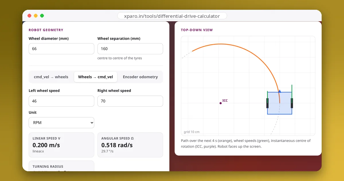
Most mobile robots, from robot vacuums to warehouse carts, steer the same way: two driven wheels on one axle, turning at different speeds. The relationship between the wheel speeds and the robot's motion is called differential-drive kinematics. It takes four lines of algebra, and once you can derive them yourself, motor drivers, odometry and controller configuration all make more sense.
The setup
Two wheels of radius r sit on a common axle, a distance L apart (the wheel separation, measured between the centres of the tyres' contact patches). Casters or ball rollers carry the rest of the weight. Following ROS conventions, the robot's X axis points forward and Y to the left, and positive turning is counter-clockwise seen from above.
The robot's motion in the plane is fully described by two numbers, which are exactly the two fields a ROS Twist command uses for a ground robot:
- v: linear speed forward (m/s),
linear.x - ω: angular speed (rad/s),
angular.z
The key idea: rotation about a point
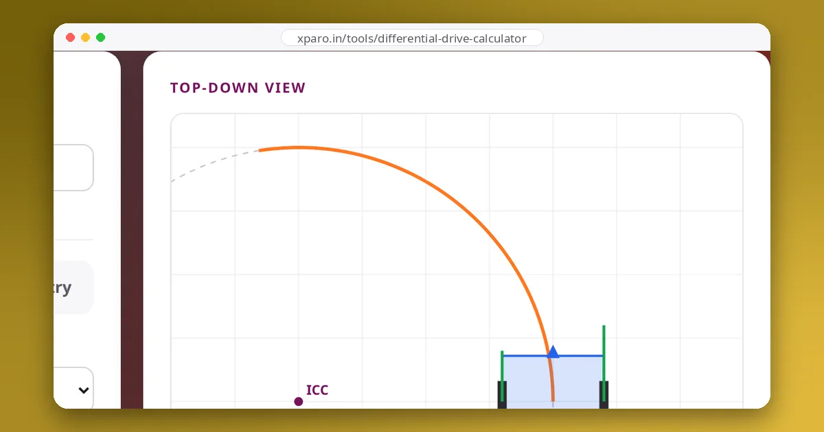
At any instant, a differential-drive robot is rotating about a point on the line through its axle, the instantaneous centre of rotation (ICC). Both wheels trace circles around it. The wheel on the outside of the turn has a longer circle to cover, so it must move faster. If the ICC is a distance R from the middle of the axle (positive to the left), the wheels are at R − L/2 and R + L/2 from it, and everything turns at the same angular speed ω:
Inverse kinematics: from v and ω to wheel speeds
Substituting R = v ÷ ω gives the equations every differential-drive motor driver implements:
Forward kinematics: from wheel speeds to v and ω
Solving the same equations the other way gives the robot's motion from measured wheel speeds, the basis of wheel odometry:
The linear speed is the average of the wheels; the turning rate is their difference divided by the separation.
A worked example
A robot with 100 mm wheels (r = 0.05 m) 300 mm apart receives linear.x = 0.5 and angular.z = 1.0:
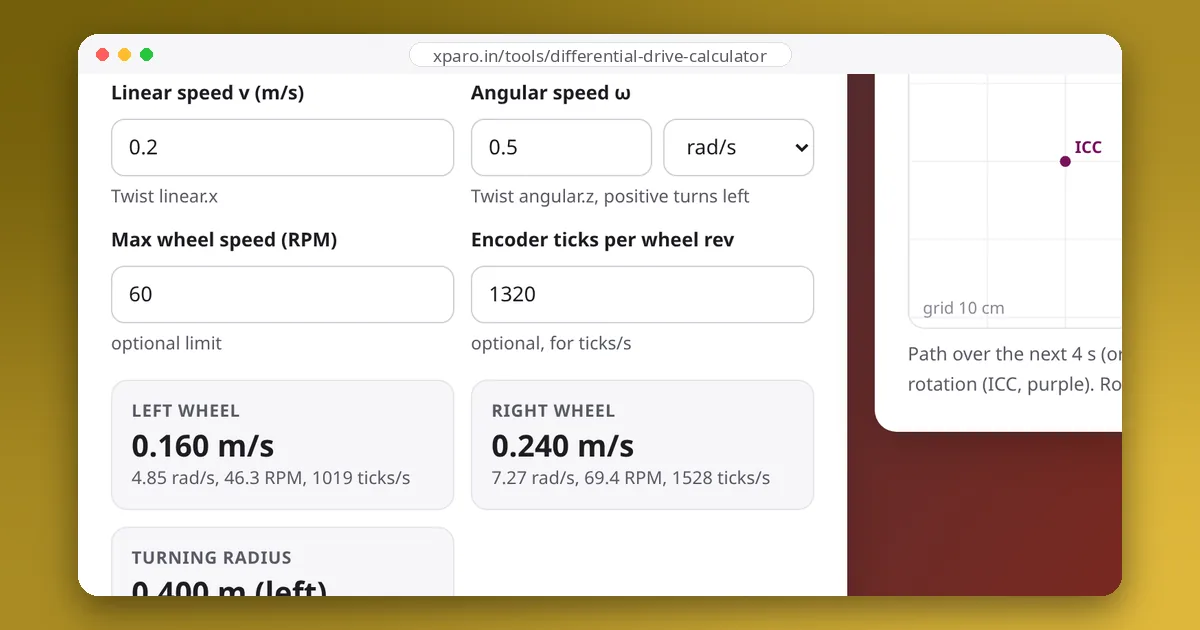
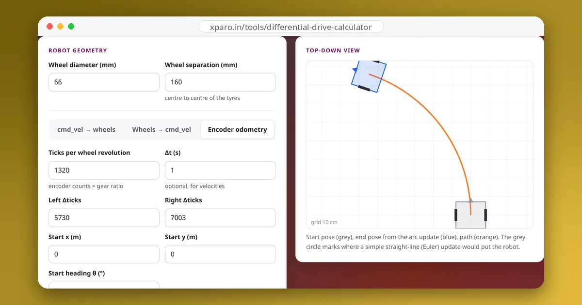
Check it the other way: (0.65 + 0.35) ÷ 2 = 0.5 m/s and (0.65 − 0.35) ÷ 0.3 = 1.0 rad/s. The Differential Drive Calculator runs both directions and draws the resulting path and ICC.
Special cases worth knowing
| Motion | Wheels | v, ω | R |
|---|---|---|---|
| Straight line | equal speeds | v ≠ 0, ω = 0 | infinite |
| Spin on the spot | equal and opposite | v = 0, ω ≠ 0 | 0 |
| Pivot about one wheel | one wheel stopped | v = ±ω × L/2 | L/2 |
| Gentle curve | similar speeds | small ω | large |
The ability to spin on the spot is why differential drive is so popular indoors: the robot can turn to any heading in its own footprint. The price is that it cannot move sideways (it is non-holonomic), so parking next to a shelf takes a manoeuvre.
What the equations assume
- No slip. The wheels roll without skidding. Hard acceleration, smooth floors and ramps break this, which is why odometry drifts.
- Known r and L. The effective values, which differ from the nominal ones because tyres compress and contact patches have width. Calibrate them, as in our calibration guide.
- Two wheels. Four-wheel skid-steer robots behave approximately like differential drive with a larger effective separation, because their wheels must scrub sideways to turn.
Where to go next
To see these equations inside ROS 2, read from cmd_vel to wheel speeds. To turn encoder counts into position, read wheel odometry from encoder ticks.