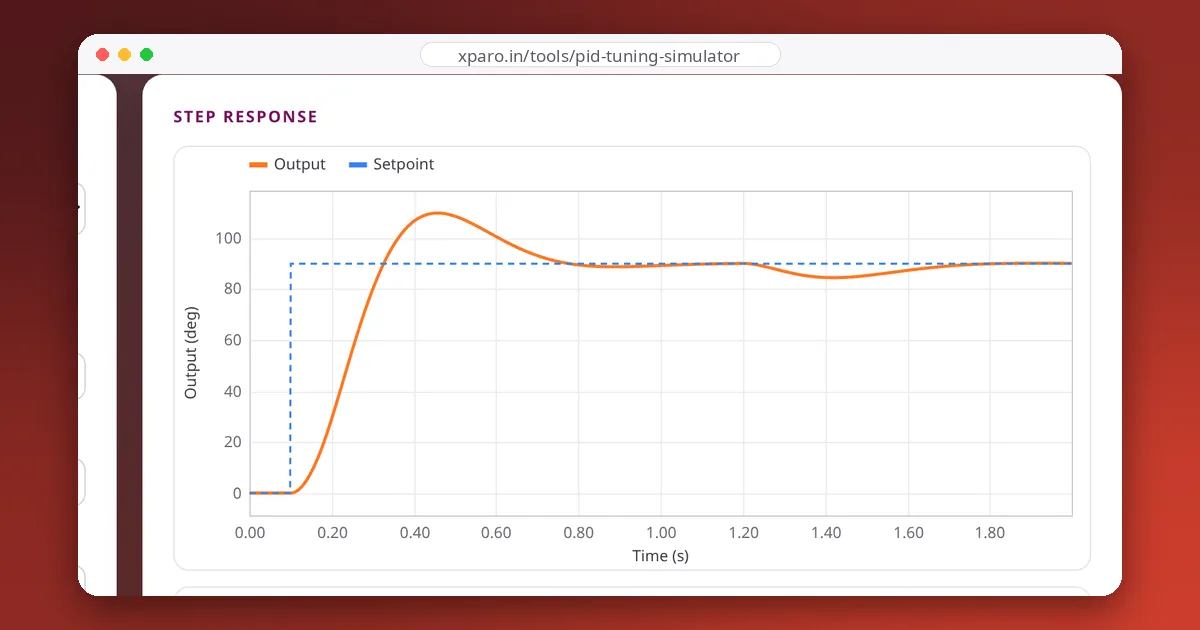
PID control is how most robots hold a wheel at a set speed, an arm at a set angle, or a heading on a straight line. The algorithm fits in a dozen lines of code, yet it is the source of endless head-scratching when a robot oscillates, overshoots or never quite reaches its target. This guide builds an intuition for what each of the three terms does, then turns it into code you can use.
The problem PID solves
You want something on the robot to reach a target and stay there: a wheel at 100 RPM, a gripper at 30°, a battery heater at 25 °C. You can measure where it is and you can push it (with voltage, force or power), but you don't know exactly how hard to push, because the load, the friction and the battery voltage keep changing. A feedback controller solves this by measuring the error, the difference between the target (the setpoint) and the measurement, and pushing in proportion to what it sees, many times per second.
The equation
The controller output u is the sum of three terms, each with its own gain. In words: push in proportion to the error now (P), to the error accumulated over time (I), and to how fast the error is changing (D).
P: react to the present
The proportional term pushes harder the further you are from the target. Raising Kp makes the response faster, but past a point it overshoots and rings, because the system has inertia and delay: by the time the error reaches zero, it is already moving fast.
P alone usually leaves a steady-state error. A motor needs some voltage just to keep turning against friction and load, and with P alone that voltage can only come from a remaining error. In the PID Tuning Simulator's motor speed loop (15 RPM per volt), Kp = 0.3 settles at about 81.8 RPM instead of 100. The arithmetic is exact: the remaining error is 100 ÷ (1 + 0.3 × 15) ≈ 18.2 RPM.
I: remember the past
The integral term adds up the error over time and keeps growing as long as any error remains. It is what removes the steady-state error: in the simulator, adding Ki = 6 to the same motor loop brings it to exactly 100 RPM with under 2 % overshoot, settling in about 0.15 s.
The price of the integral is memory. It keeps pushing after the error has changed sign, so too much Ki causes overshoot and slow oscillation. And if the actuator saturates, the integral keeps growing while the output cannot respond, a problem called integral windup.
D: anticipate the future
The derivative term reacts to how fast the error is changing. As the output rushes toward the target, the error shrinks quickly, the derivative is large and negative, and D brakes the approach. That is damping: D lets you use more P without overshoot. In the simulator's lightly damped mass-on-a-spring, the same P and I gains ring for seconds without D and settle cleanly with it.
D has a weakness: it amplifies noise, because noise changes fast. A real implementation filters the derivative and usually takes it from the measurement rather than the error, as the code below does.
What each gain does, at a glance
| Raise… | Rise time | Overshoot | Settling | Steady-state error |
|---|---|---|---|---|
| Kp | faster | more | small change | smaller (rarely zero) |
| Ki | faster | more | slower if too high | removed |
| Kd | small change | less | faster | no effect |
These are tendencies, not laws. Too much of any gain eventually makes things worse, and gains interact.
A PID controller in Python
This version adds the three details that separate a textbook PID from one that behaves on a robot: output limits, clamping anti-windup, and a filtered derivative taken from the measurement.
class PID:
    def __init__(self, kp, ki, kd, out_min, out_max, d_filter_tau=0.0):
        self.kp, self.ki, self.kd = kp, ki, kd
        self.out_min, self.out_max = out_min, out_max
        self.tau = d_filter_tau
        self.integral = 0.0
        self.d_term = 0.0
        self.prev_measurement = None

    def update(self, setpoint, measurement, dt):
        error = setpoint - measurement
        p_term = self.kp * error

        # derivative of the measurement: no spike when the setpoint jumps
        if self.prev_measurement is None:
            self.prev_measurement = measurement
        d_raw = -self.kd * (measurement - self.prev_measurement)
        self.d_term = (self.tau * self.d_term + d_raw) / (self.tau + dt)
        self.prev_measurement = measurement

        # integrate unless the output is saturated and the error pushes further
        candidate = self.integral + self.ki * error * dt
        unclamped = p_term + candidate + self.d_term
        if not ((unclamped > self.out_max and error > 0) or
                (unclamped < self.out_min and error < 0)):
            self.integral = candidate

        output = p_term + self.integral + self.d_term
        return max(self.out_min, min(self.out_max, output))
Call update at a fixed rate with the time step dt in seconds. We tested this class against the motor model above: with Kp = 0.3 and Ki = 6 it settles at 100 RPM with about 2 % overshoot, holding 6.67 V, exactly 100 ÷ 15.
Where PID shows up on a robot
- Wheel speed: the inner loop of almost every mobile robot; see closed-loop motor speed control.
- Joint position: servos and arms.
- Heading and line following: steering toward a direction or a line.
- Temperature, pressure, altitude: anything with a sensor and an actuator.
Try it
Reading about PID only goes so far. Open the PID Tuning Simulator, pick the motor speed loop, and use the presets to see each effect described here: the steady error of P alone, the integral fixing it, windup, and derivative damping. Then follow our step-by-step tuning method.