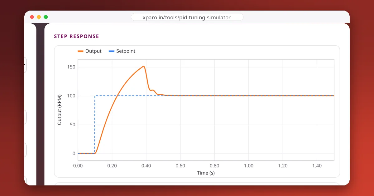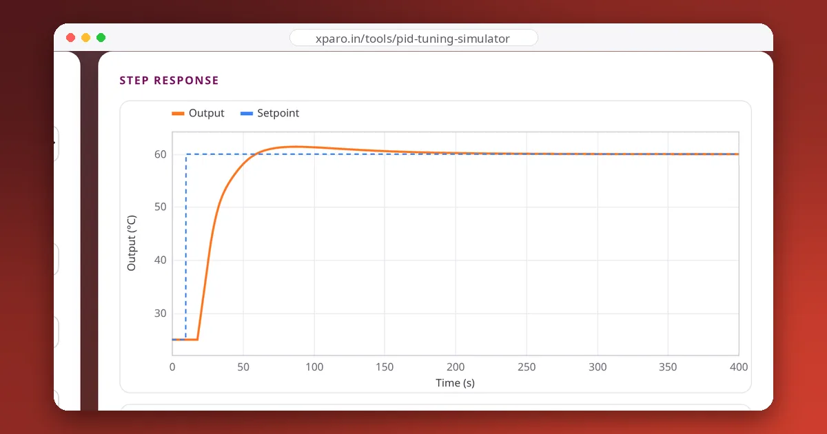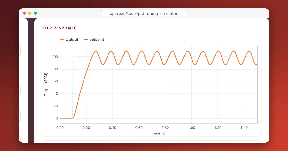
Most PID tuning on robots is done by hand, and most hand tuning is done badly: three gains changed at once, by guesswork, until something looks roughly right. A simple, repeatable method gets better results faster. This guide lays one out and works through it on the motor position loop in our PID Tuning Simulator, with the numbers it produced at every step.
Before you touch a gain
- Make it safe. Put a wheeled robot on blocks, limit an arm's travel, and know how to cut power. A bad gain can make a mechanism slam into its end stops.
- Fix the loop rate. Run the controller at a steady rate and compute
dtfrom it. Changing the rate later changes the effective gains. - Get the sign right. With a small Kp, a positive error must push the output toward the setpoint. If the system runs away, flip the sign of the output, not the gains.
- Clamp the output to what the actuator can take and turn on anti-windup from the start.
- Log and plot. You cannot tune what you cannot see. Plot setpoint, measurement and controller output against time, for example with PlotJuggler, or by printing values to the Web Serial Monitor's plotter.
- Use a repeatable test. The same step every time, from the same starting point, so you compare like with like.
Step 1: P only
Set Ki and Kd to zero. Start with a small Kp and double it after each test until the response is quick and overshoots slightly. Changing gains by factors, not fixed amounts, gets you to the right order of magnitude quickly.
On the simulator's position loop (a motor turning a shaft to 90°, with a 12 V driver):
| Kp (V per degree) | Rise time | Overshoot |
|---|---|---|
| 0.02 | 915 ms | 0 % |
| 0.05 | 340 ms | 9 % |
| 0.10 | 195 ms | 23 % |
| 0.20 | 136 ms | 34 % |
Beyond about 0.2, the driver spends most of the move at its 12 V limit, so more Kp buys little speed and only more overshoot. That tells you where the useful range ends. Pick a value with some overshoot; we continued with 0.22.
Step 2: add D to calm the overshoot
Raise Kd from zero until the overshoot shrinks to what you can accept. Too much D makes the response sluggish and, on real hardware, amplifies sensor noise into a buzzing actuator.
| Kd (Kp = 0.22) | Overshoot | Settling time (2 %) |
|---|---|---|
| 0.005 | 22 % | 0.75 s |
| 0.010 | 12 % | 0.52 s |
| 0.020 | 0.8 % | 0.35 s |
| 0.040 | 0 % | 0.82 s (over-damped) |
Kd = 0.02 is the sweet spot: almost no overshoot and the fastest settling. Doubling it again slows everything down. If the plotted output gets noisy as you raise Kd, increase the derivative filter time constant before giving up on D.
Step 3: add I only as much as you need
Now apply a disturbance: a load that pushes back. In the simulator, turn on the load disturbance. With PD alone, the shaft settles about 9° short under load, because only a lasting error can produce the extra voltage the load needs. The integral term removes that error.
| Ki (Kp = 0.3, Kd = 0.02) | Error left under load | Setpoint overshoot |
|---|---|---|
| 0 (PD) | 6.7° | 4 % |
| 0.6 | 1.6° | 14 % |
| 1.2 | 0.16° | 22 % |
| 2.4 | 0.34°, still oscillating | 35 % |
Notice the trade-off: in a position loop, the motor already integrates speed into angle, so adding I always costs some overshoot on setpoint changes. Choose the smallest Ki that removes the load error in acceptable time. If the overshoot is a problem, common remedies are to integrate only near the target, to ramp the setpoint instead of stepping it, or to add a feedforward term for a known load so the integral has less to do.
Step 4: stress test
- Different step sizes. Small steps behave differently from large ones that saturate the actuator.
- Disturbances. Push the mechanism, add the real payload, drive on carpet.
- Noise. Watch the controller output, not just the measurement: a smooth position with a buzzing motor current is not a good tuning.
- The whole operating range. A loop tuned at full battery may oscillate on a flat one, because the actuator gain changes with voltage.
Reading the symptoms
| Symptom | Likely cause | Try |
|---|---|---|
| Slow, never quite reaches the target | Kp too low, no I | Raise Kp, add a little Ki |
| Fast oscillation around the target | Kp too high, or not enough D | Lower Kp or add Kd |
| Slow, wide oscillation | Ki too high | Lower Ki |
| Big overshoot after a long saturated move | Integral windup | Enable anti-windup |
| Noisy, buzzing output | Kd too high or unfiltered | Filter D, lower Kd |
| Behaves well in one direction only | Friction or a load that differs by direction | Feedforward, or tune for the worse direction |
When to use a formula instead
Hand tuning works well when tests are quick and safe. For slow processes, or when you need a starting point in one experiment, tuning rules such as Ziegler-Nichols compute gains from a single test. They tend to be aggressive; our guide to Ziegler-Nichols tuning shows how they compare in practice. And make sure the implementation itself is sound before blaming the gains: see integral windup, derivative kick and noise.