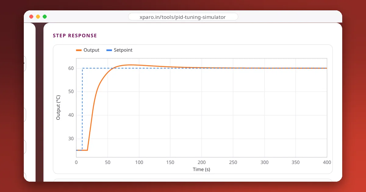
The Ziegler-Nichols rules, published in 1942, turn one simple experiment into a full set of PID gains. They are still the first tuning method most engineers learn, and still a reasonable starting point. They are also famously aggressive. This guide explains both versions of the method, applies them to the heater in our PID Tuning Simulator, and compares the results with two gentler modern rules.
The test system
The simulator's heater behaves like many slow processes: a first-order lag with a time constant of 60 s, a gain of 1.5 °C per percent of heater power, and 8 s of dead time (the delay before a change in power shows up in the measurement). The task is to raise the temperature from 25 °C to 60 °C, with the heater limited to 0 to 100 % power.
Method 1: the ultimate gain (closed loop)
- Use P control only (Ki = Kd = 0).
- Increase Kp until the output oscillates steadily, neither growing nor dying away. That gain is the ultimate gain Ku.
- Measure the period of the oscillation, Tu.
- Compute the gains from the table.
| Controller | Kp | Ti | Td |
|---|---|---|---|
| P | 0.5 Ku | ||
| PI | 0.45 Ku | Tu ÷ 1.2 | |
| PID | 0.6 Ku | 0.5 Tu | 0.125 Tu |
The table gives the integral and derivative as times. For the parallel form used in the simulator and most code (u = Kp·e + Ki·∫e + Kd·de/dt), convert with Ki = Kp ÷ Ti and Kd = Kp × Td.
For our heater model, the point of steady oscillation can be calculated exactly: it is where the lag and the dead time together delay the signal by half a cycle. That gives Ku ≈ 8.28 (percent per °C) and Tu ≈ 30.4 s. The Ziegler-Nichols PID gains are then:
Method 2: the step response (open loop)
If you can't safely make a system oscillate, use its open-loop step response instead. Apply a step in the controller output, record the measurement, and read off three numbers: the process gain K (change in output divided by change in input), the apparent dead time L, and the time constant T. For the heater, K = 1.5, L = 8 s and T = 60 s.
| Controller | Kp | Ti | Td |
|---|---|---|---|
| P | T ÷ (K·L) | ||
| PI | 0.9 T ÷ (K·L) | L ÷ 0.3 | |
| PID | 1.2 T ÷ (K·L) | 2 L | 0.5 L |
For the heater: PID Kp = 1.2 × 60 ÷ (1.5 × 8) = 6.0, Ti = 16 s (Ki = 0.375) and Td = 4 s (Kd = 24).
How they perform
We ran each set of gains in the simulator, with anti-windup on, derivative on measurement, the heater's real power limit, and then again with a sudden 10 % loss of heater power (a draught) to test disturbance rejection:
| Rule | Kp | Ki | Kd | Overshoot | Settling (2 %) | Worst dip after the draught |
|---|---|---|---|---|---|---|
| ZN closed-loop PID | 4.97 | 0.327 | 18.9 | 9.3 % | 62 s | 2.3 °C |
| ZN closed-loop PI | 3.73 | 0.147 | 0 | 11.9 % | 69 s | 2.8 °C |
| ZN open-loop PID | 6.00 | 0.375 | 24.0 | 10.5 % | 161 s | 2.5 °C |
| ZN open-loop PI | 4.50 | 0.169 | 0 | 14.2 % | 99 s | 2.7 °C |
| Tyreus-Luyben PI | 2.59 | 0.039 | 0 | 1.8 % | 92 s | 3.3 °C |
| SIMC PI (τc = θ) | 2.50 | 0.042 | 0 | 5.1 % | 49 s | 3.3 °C |
Two things stand out. First, the Ziegler-Nichols gains reject disturbances best, which is what they were designed for, but they overshoot and ring more. Second, the actuator limit and anti-windup tame them considerably here. Without anti-windup, the same ZN PID gains overshoot by 73 % and take 146 s to settle, which is closer to the behaviour people usually associate with Ziegler-Nichols.
The gentler alternatives
- Tyreus-Luyben uses the same experiment as closed-loop ZN but with smaller gains (for PI: Kp = Ku ÷ 3.2, Ti = 2.2 Tu). It gives very little overshoot at the cost of slower disturbance recovery.
- SIMC (Skogestad's rules) uses the step-response model: Kp = (1 ÷ K) × T ÷ (τc + L) and Ti = min(T, 4(τc + L)), where τc is the closed-loop response time you want. Choosing τc = L is a robust default; in our test it settled fastest of all.
When Ziegler-Nichols fails
- Systems you can't push into oscillation safely, which includes most robot joints and anything carrying people.
- Integrating processes such as position loops, where the open-loop step response never levels off.
- Very long dead time compared with the time constant: the rules become too aggressive.
- Noisy measurements: the derivative gains from ZN are large and amplify noise; our guide to real-world PID problems shows how much.
- Strongly non-linear actuators: friction, backlash and saturation break the linear assumptions the rules rely on.
How to use these rules well
Treat any tuning rule as a starting point. Apply it, look at the response, and then refine by hand, usually by lowering Kp and Ki a little, following our step-by-step tuning method. You can reproduce every row of the table above in the simulator: select the heater, type in the gains, and toggle the load disturbance and anti-windup.